Hyperparameter Optimization#
After your prototype has been verified and runs smoothly with ProtoTrainer, you can scale it to an ablation study, perform parallel hyperparameter optimization, and analyze the results with Ablator.
In this chapter, we will learn how to set up and launch a parallel ablation experiment for an ablation study with Ablator.
Similarly to launching a prototype experiment, here there are also 3 main steps to run an ablation experiment in ablator:
Configure the experiment.
Create model wrapper that defines boiler-plate code for training and evaluating models.
Create the trainer and launch the experiment.
Recall from the Introduction tutorial, Ablator combines Optuna for hyperparameter optimization (HPO) and Ray back-end for parallelizing the trials. So, an extra step is to start a ray cluster before launching the experiment.
Let us first import all necessary dependencies:
from ablator import ModelConfig, OptimizerConfig, TrainConfig, RunConfig, ParallelConfig
from ablator import ModelWrapper, ParallelTrainer, configclass
from ablator.config.hpo import SearchSpace

import torch
import torch.nn as nn
import torch.optim as optim
from torch.utils.data import DataLoader, Dataset
import torchvision
import torchvision.transforms as transforms

import os
import shutil
from sklearn.metrics import f1_score, accuracy_score
Launch the parallel experiment#
Configure the experiment#
We will follow exactly the same steps as in the tutorial on Prototyping models to configure the experiment:
Here’s a summary of how we will configure it:
Model Configuration: defines hyperparameters for the number of filters and activation function.
Optimizer Configuration: adam (lr = 0.001).
Train Configuration:
batch_size = 32,epochs = 10, random weights initialization is set as true.Runing Configuration: GPU as hardware, a random seed for the experiment. We let the experiment runs HPO for
total_trials = 20trials, allowingconcurrent_trials = 2trials to run in parallel. We also use a HPO search space for the model and the optimizer, and use validation loss as the metric to optimize, in specific, we want to minimize this ({"val_loss": "min"}).
Configure the model#
Model configuration#
For the model configuration, we defines the following hyperparameters:
num_filter1,num_filter2(integer): number of filters at each convolutional layeractivation(string): activation function to use in layers.
@configclass
class CustomModelConfig(ModelConfig):
  num_filter1: int
  num_filter2: int
  activation: str

model_config = CustomModelConfig(
    num_filter1 =32,
    num_filter2 = 64,
    activation = "relu"
)
Since the hyperparameters are defined using primitive data types (aka Stateful), we must provide concrete values when initializing the model_config object.
Creating Pytorch CNN Model#
We define a custom CNN model FashionCNN with the following architecture:
The first convolutional layer: takes a single channel and applies
num_filter1filters to it. Then, applies an activation function and a max pooling layer.The second convolutional layer: takes
num_filter1channels and appliesnum_filter2filters to them. It also utilizes an activation function and a pooling layer.The third convolutional layer: This is an additional layer that applies
num_filter2filters.A flattening layer: converts the convolutional layers into a linear format and subsequently produces a 10-dimensional output for labeling.
FashionCNN is then included in MyModel as a sub-module. MyModel’s forward function performs forward computation, add a loss function, and returns the predicted labels and loss during model training and evaluation.
# Define the model
class FashionCNN(nn.Module):
    def __init__(self, config: CustomModelConfig):
        super(FashionCNN, self).__init__()

        activation_list = {"relu": nn.ReLU(), "elu": nn.ELU(), "leakyRelu": nn.LeakyReLU()}

        num_filter1 = config.num_filter1
        num_filter2 = config.num_filter2
        activation = activation_list[config.activation]

        self.conv1 = nn.Conv2d(1, num_filter1, kernel_size=3, stride=1, padding=1)
        self.act1 = activation
        self.maxpool1 = nn.MaxPool2d(kernel_size=2, stride=2)

        self.conv2 = nn.Conv2d(num_filter1, num_filter2, kernel_size=3, stride=1, padding=1)
        self.act2 = activation
        self.maxpool2 = nn.MaxPool2d(kernel_size=2, stride=2)

        self.conv3 = nn.Conv2d(num_filter2, num_filter2, kernel_size=3, stride=1, padding=1)
        self.act3 = activation

        self.flatten = nn.Flatten()
        self.fc1 = nn.Linear(num_filter2 * 7 * 7, 10)


    def forward(self, x):
        x = self.conv1(x)
        x = self.act1(x)
        x = self.maxpool1(x)
        x = self.conv2(x)
        x = self.act2(x)
        x = self.maxpool2(x)
        x = self.conv3(x)
        x = self.act3(x)
        x = self.flatten(x)
        x = self.fc1(x)

        return x

class MyModel(nn.Module):
    def __init__(self, config: CustomModelConfig) -> None:
        super().__init__()

        self.model = FashionCNN(config)
        self.loss = nn.CrossEntropyLoss()

    def forward(self, x, labels=None):
        out = self.model(x)
        loss = None

        if labels is not None:
            loss = self.loss(out, labels)
            labels = labels.reshape(-1, 1)

        out = out.argmax(dim=-1)
        out = out.reshape(-1, 1)

        return {"y_pred": out, "y_true": labels}, loss
Configure the training process#
optimizer_config = OptimizerConfig(
    name="adam",
    arguments={"lr": 0.001}
)

train_config = TrainConfig(
    dataset="Fashion-mnist",
    batch_size=32,
    epochs=10,
    optimizer_config=optimizer_config,
    scheduler_config=None,
    rand_weights_init = True
)
Configure the running configuration#
To run an ablation study, we need to specify a search space for the hyperparameters of interest. This search space will then be used to configure the running configuration.
Search Space#
For this tutorial, we have defined search_space object for four different hyperparameters:
Number of filters in the first and second convolutional layers: range between 32 and 64, and 64 and 128, respectively.
The activation function to use: any of
relu,elu, andleakyRelu.Learning rate value: ranges between 1e-3 and 1e-2.
search_space = {
    "model_config.num_filter1": SearchSpace(value_range = [32, 64], value_type = 'int'),
    "model_config.num_filter2": SearchSpace(value_range = [64, 128], value_type = 'int'),
    "train_config.optimizer_config.arguments.lr": SearchSpace(
        value_range = [0.001, 0.01],
        value_type = 'float'
        ),
    "model_config.activation": SearchSpace(categorical_values = ["relu", "elu", "leakyRelu"]),
}
Parallel Configuration#
As the last step to configure the experiment, we pass search_space, train_config, and model_config to the ParallelConfig. Other parameters are also set:
@configclass
class CustomParallelConfig(ParallelConfig):
  model_config: CustomModelConfig

parallel_config = CustomParallelConfig(
    train_config=train_config,
    model_config=model_config,
    metrics_n_batches = 800,
    experiment_dir = "/tmp/experiments/",
    device="cuda",
    amp=True,
    random_seed = 42,
    total_trials = 20,
    concurrent_trials = 5,
    search_space = search_space,
    optim_metrics = {"val_loss": "min"},
    gpu_mb_per_experiment = 1024,
)
Note
We recommend that the experiment directory
ParallelConfig.experiment_dirshould be an empty directory.Make sure to redefine the running configuration class to update its
model_configattribute fromModelConfig(by default) toCustomModelConfigbefore creating the config object.
Create the model wrapper#
The model wrapper class ModelWrapper serves as a comprehensive wrapper for PyTorch models, providing a high-level interface for handling various tasks involved in model training. It defines boiler-plate code for training and evaluating models, which significantly reduces development efforts and minimizes the need for writing complex code, ultimately improving efficiency and productivity:
It takes care of creating and utilizing data loaders, evaluating models, importing parameters from configuration files into the model, setting up optimizers and schedulers, and checkpoints, logging metrics, handling interruptions, and much more.
Its functions are over-writable to support for custom use-cases (read more about these functions in this documentation of Model Wrapper).
An important function of the ModelWrapper is make_dataloader_train, which is used to create a data loader for training the model. In fact, you must provide a train dataloader to make_dataloader_train before launching the experiment.
Therefore, we will start prepare the datasets first. Then, we write some eluation functions to be used to evaluate our model. Finally, we will create the model wrapper and train the model.
Prepare the dataset#
Fashion MNIST is a dataset consisting of 60,000 grayscale images of fashion items. The images are categorized into ten classes, which include clothing items.
Image dimensions: 28 pixels x 28 pixels (grayscale)
Shape of the training data tensor: [60000, 1, 28, 28]
Here we will create two datasets: one for training and one for validation.
transform = transforms.ToTensor()

train_dataset = torchvision.datasets.FashionMNIST(
    root='./data',
    train=True,
    download=True,
    transform=transform
)

test_dataset = torchvision.datasets.FashionMNIST(
    root='./data',
    train=False,
    download=True,
    transform=transform
)
Create the Model Wrapper#
We will now create a model wrapper class and overwrite the following functions. Note that the ModelWrapper will be similar to that in Prototyping models tutorial.
make_dataloader_trainandmake_dataloader_val: to provide the training dataset and validation dataset as dataloaders (In PyTorch, a DataLoader is a utility class that provides an iterable over a dataset. It is commonly used for handling data loading and batching in machine learning and deep learning tasks).evaluation_functions: to provide the evaluation functions that will evaluate the model on the datasets. In this function, you must return a dictionary of callables, where the keys are the names of the evaluation metrics and the values are the functions that compute the metrics.
class MyModelWrapper(ModelWrapper):
    def __init__(self, *args, **kwargs):
        super().__init__(*args, **kwargs)

    def make_dataloader_train(self, run_config: CustomParallelConfig):
        return torch.utils.data.DataLoader(
            train_dataset,
            batch_size=32,
            shuffle=True
        )

    def make_dataloader_val(self, run_config: CustomParallelConfig):
        return torch.utils.data.DataLoader(
            test_dataset,
            batch_size=32,
            shuffle=False
        )

    def evaluation_functions(self):
        return {
            "accuracy": lambda y_true, y_pred: accuracy_score(y_true.flatten(), y_pred.flatten()),
        }
Now create the model wrapper object, passing the model class as its argument:
wrapper = MyModelWrapper(
    model_class=MyModel,
)
Create the trainer and launch the experiment with ParallelTrainer#
ParallelTrainer, an extention from ProtoTrainer, is responsible for creating and pushing trials to the Ray cluster for parallelization of the ablation study.
We first initialize the trainer, providing it with the model wrapper and the running configuration.
Next, call the
launch()method, passing toworking_directorythe path to the main directory that you’re working at (which stores codes, modules that will be pushed to ray).
ablator = ParallelTrainer(
    wrapper=wrapper,
    run_config=parallel_config,
)

ablator.launch(working_directory = os.getcwd())
Note
By default,
ablator.launch(working_directory = os.getcwd())will initialize a ray cluster on your machine, and this cluster will be used for the experiment.You have the option to scale the experiment to a cluster that’s running somewhere else (e.g. on a cloud service like AWS). Given a ray cluster, you can use
ablator.launch(working_directory = os.getcwd(), ray_address = <address>)to launch the experiment on that cluster.To learn about running ablation experiments on cloud ray clusters, refer to Launch-in-cloud-cluster tutorial.
We can provide resume = True to the launch() method to resume training the model from existing checkpoints and existing experiment state. Refer to the Resume experiments tutorial for more details.
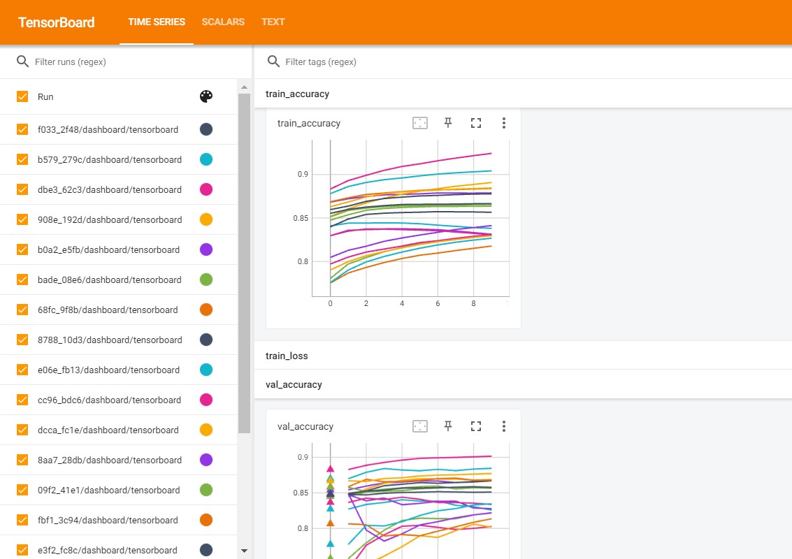
Visualizing experiment results in TensorBoard#
Since ablator automatically stores TensorBoard events files for each training process, we can perform a short visualization with TensorBoard to compare how trials perform:
Install
tensorboardand load using%load_ext tensorboardif using a notebook.Run the command
%tensorboard --logdir <experiment_dir>/experiments_<experiment id> --port [port], where<experiment_dir>is the experiment directory that we passed to the parallel config (parallel_config.experiment_dir = "/tmp/experiments/"), andexperiments_<experiment id>is generated by ablator.
%load_ext tensorboard
%tensorboard --logdir /tmp/experiments/ --port 6008
More detailed analysis for ablation studies will be explored in later tutorials.
Finally, after completing all the trials, metrics obtained in each trial will be stored in the experiment_dir. This directory contains subdirectories representing the trials, as well as SQLite databases for Optuna and the experiment’s state.
Components stored in each trial directory are: best_checkpoints, checkpoints, results, training log, configurations, and metadata.
To learn more, you can read the Experiment output directory tutorial, which explains the content of the experiment directory in detail.
In the next tutorial, we will learn how to analyze the results from the trained trials.